This article considers the problem of soil-structure interaction in foundation design and how to carry out the analysis of a beam on elastic foundation.
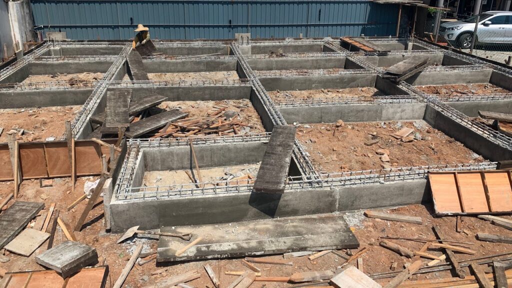
Many problems in geotechnical engineering problems can be idealized as a beam on elastic foundation problem. Recall that in the analysis of spread foundations, particularly raft foundations, two approaches can be adopted – the rigid approach that considers the foundations to be relative stiff thereby neglecting the elastic properties of the soil and the flexible approach that considers it.
To properly analyse and design a raft foundation or foundation element that is in direct contact with a soil, the elastic properties of the soil need to be cognized. This is in other words referred to as the soil-structure interaction phenomenon, whereby the behaviour of a structure is not only influenced by its own properties but by the properties of the surrounding soil or foundation materials. One of the methods available for resolving this problem is by the analysis of beams on elastic foundation.
This article presents the analysis of beams on elastic foundations. It aims to provide a background on the subject and a suitable analysis method for hand calculations.
Beams on Elastic Foundation
When a beam sits on an elastic foundation and it is under the influence of external loads, the beam develops continuous reactions that are proportional at each location along the beam to the deflection of the beam at the location. This is the reason for the name ‘elastic foundation.’
Several models have been provided for the analysis of a beam on elastic foundation. For the analytical procedure, the most popular being the one proposed by Winkler (1867) or for the numerical methods through the use of finite element analysis. In this article the former is considered.
Winkler-Bach Theory
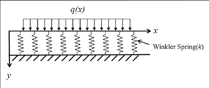
The Winkler-Bach theory, also known as the beam-on-elastic-foundation model, is a simplified approach used to analyse the behaviour of beams supported by elastic foundations. This theory assumes that the foundation behaves like a series of independent linear springs (See Figure 1) distributed along the length of the beam. Each spring represents the stiffness of the foundation material beneath the beam. The Winkler-Bach theory provides a practical and computationally efficient method for estimating the deflections and stresses in beams resting on elastic foundations.
It’s however, important to note that the Winkler-Bach theory simplifies the actual soil-structure interaction by assuming linear elastic behaviour and neglecting certain factors such as soil nonlinearity and spatial variability. But despite its simplifications, the theory provides valuable insights into the behaviour of beams on elastic foundations and serves as a foundational concept on the subject.
Mathematically, the Winkler-Bach theory can be expressed using the following equations:
Force-Deflection Relationship
The foundation stiffness, represented by the spring constant k, relates the applied force F to the resulting deflection δ. This relationship is analogous to Hooke’s Law for linearly elastic materials.
F = k \times \delta
Bending Moment Equation:
For a beam subjected to distributed loading, the bending moment M at any point along the beam can be expressed in terms of the beam’s flexural rigidity EI and the curvature θ:
M=EI \frac{d^2 \theta}{dx^2}Beam Equation with Foundation Reaction:
Incorporating the foundation reaction due to the elastic support, the differential equation governing the beam’s deflection becomes:
\frac{d^4w}{dx^4} =\frac{M}{EI} + \frac{k}{EI} .wWhere:
- w(x) is the deflection of the beam at position x,
- M is the bending moment along the beam,
- EI is the flexural rigidity of the beam,
- ks is the spring constant of the elastic foundation.
Solving the above differential equation yields the deflection function w(x) for the beam on an elastic foundation. By applying appropriate boundary conditions, such as fixed or simply supported ends, engineers can determine the deflections, bending moments, and other relevant structural responses.
Analysis of Beams on Elastic Foundations (Warren & Richard, 2002)
Several attempts were made to simplify the solution to the differential equation and by extension the problem of beams on elastic foundation. For instance, Warren & Richard (2002) published tables and equations that can be used to quickly analyse a beam on elastic foundation.
Table 8.5 of Warren & Richard (2002) which is reproduced belwo provides equations that can be used to determine the reactions and deflections occurring at the initial end of a finite-length beam resting on an elastic foundation. Additionally, it supplies equations for the shear, moment, slope, and deflection at any position x along the beam’s length. These formulas are structured to streamline implementation in programming for digital computers or programmable calculators.
In principle, the equations delineated in Table 8.5 hold true for any finite-length beam or finite foundation modulus. However, practical application should avoid instances where the parameter βl exceeds 6. This caution arises from potential roundoff errors, particularly when subtracting two closely comparable large numbers, compromising the reliability of the analysis result. Consequently, Table 8.6 containing formulas tailored for semi-infinite and infinite-length beams on elastic foundations. These formulations are simpler, assuming that the beam’s far end remains distant enough to exert negligible influence on the response of the initial end to loading. This assumption holds when βl > 6 and the load is closer to the initial end.
Tables 8.3 and 8.4 are also provided to aid in solving the formulas from Table 8.5 & 8.6 allowing for interpolation of included values. However, caution is advised when encountering large and nearly equal number differences. For a beam with a single load, a more reliable interpolation method involves solving the problem twice, shifting the load to the left and right until βl value from Table 8.3 is attained, then performing linear interpolation between these solutions.
Presenting the formulas for end reactions and displacements in terms of constants Ci and Cai in Table 8.5 offers the advantage of direct determination of loads anywhere on the span. Simplifying the formulas is feasible when loads are concentrated at the initial end (i.e., a ¼ 0), aligning Ci with Cai. To ease the use of Table 8.5 for cases with concentrated loads, moments, angular rotations, or lateral displacements at the initial end, equations are provided to simplify the numerators.
Worked Example
A rectangular concrete beam measuring (Figure 2) 900mm deep 500mm wide lies atop a uniform soil with a modulus of subgrade reaction (ks) of 15000 kN/m²/m. This beam spans 10m and sustains a partially distributed load of W = 100kN/m over 5m span. Assuming the self-weight of the beam is disregarded and assuming freely supported ends, Determine the bending moment at the midpoint of the partially distributed load location Use the modulus of elasticity of concrete (Ec) as 22 x 10^6 kN/m².
Check the Value of βl
\beta=(\frac{bk_s}{4EI})^{1/4}We must determine the value of the second moment area of cross-section first. Thus:
I =\frac{bh^3}{12}=\frac{0.5\times0.9^3}{12}=0.03m^4\beta=(\frac{0.5\times15000}{4\times22\times10^6\times0.03})=0.231\beta l=0.231\times10=2.31 <6
Since the Value of βl < 6 we can apply Table 8.5 for finite beam on elastic foundation supporting a partially distributed loading with freely supported end conditions. The equation for shear and bending moment, slope and deflection are as presented respectively.
Bending Moment & Shear Force Equations
V=R_AF_1- y_A2EIβ^3F_2- \theta_A2EI \beta^2F_3 -M_A\beta F_4 -\frac{w}{2\beta}F_{a2}M=M_AF_1+ \frac{R_A}{2\beta} F_2 - y_A2EIβ^2F_3- \theta_A2EI \beta F_4 -\frac{w}{2\beta^2}F_{a3}Where:
\theta_A=\frac{w}{2EI\beta^3} \frac{C_2C_{a3}-C_3C_{a2}}{C_{11}}y_A=\frac{w}{4EI\beta^4} \frac{C_4C_{a2}-2C_3C_{a3}}{C_{11}}To compute the bending moment and shear force along any point in the beam, we must determine the value of and and in turn to determine the values the following constants must be determined.
Determine Constants
C_2=cosh\beta lsin\beta l+sinh\beta lcos\beta l
=cosh2.31sin2.31+sinh2.31cos2.31 \\=0.398
C_3+sinh\beta lsin\beta l =3.69
C_4==cosh\beta lsin\beta l-sinh\beta lcos\beta l
=cosh2.31sin2.31-sinh2.31cos2.31 \\=7.125
C_{a2}= cosh\beta( l-a)sin\beta(l-a)+sinh\beta( l-a)cos\beta(l-a)=cosh1.16sin1.16+sinh1.16cos1.16 \\=2.18
C_{a3}= sinh\beta( l-a)sin\beta(l-a) =1.32C_{11}=sinh^2\beta l - sin^2 \beta l =1.89Having computed the constants, we can then compute the values of slope and deflection at point a as follows:
\theta_A=\frac{100}{2\times22\times10^6\times0.03\times0.231^3} \times\frac{0.398(1.32)-3.69(2.18)}{1.89}=-0.024rads
y_A==\frac{100}{4\times22\times10^6\times0.03\times0.231^4} \times\frac{7.13(2.18)-3.69(1.32)}{1.89}=0.075m
Bending Moment Value
Where (RA and MA = 0), If we substitute the values of slope and deflection at point A into the equations for bending moment presented above, the equation reduces as follows:
M_x=-5283F_3+7318F_4 -937F_{a3}If we substitute the equations for F3, F4 and Fa3 into the above equation, the equation further reduces to:
M_x =-5283(sinh\beta x.sin\beta x)+7318(cosh\beta xsin\beta x+sinh\beta xcos\beta x)-\\937(cosh\beta( x-a)sin\beta(x-a)+sinh\beta( x-a)cos\beta(x-a)
Since we’re required to determine the bending moment at the point of application of the partial distributed load, therefore x = 5+5/2 = 7.5m. Substituting the value of x into the above equation, yields:
M=4473kN.m
Also See: Designing a Slab-Raft Foundation | Worked Example
Sources & Citations
- Warren C.Y., Richard B. Y. (2002): Roark’s Formula for Stress and Strain (7th edition). McGraw Hill, USA (Available here: Roark’s Formulas for Stress and Strain, 8th Edition: Young, Warren and Budynas, Richard and Sadegh, Ali: Hardcover: 9780071742474: Powell’s Books (powells.com)